Point-in-Time (PIT) constructs & Join-Trees – Sonic Surf ISP| Fast Internet

Snowflake continues to set the standard for data in the cloud by removing the need to perform maintenance tasks on your data platform and giving you the freedom to choose your data model methodology for the cloud. You expect the same relational capabilities for your data model as any other platform and Snowflake helps deliver.

Data Vault models are not built for consumption by business intelligence (BI) tools, they are built for automation and agility while allowing auditability; making changes to a Data Vault model does not destroy the existing model; rather, it augments it. In order to simplify and enhance querying a Data Vault model, we will discuss why you could consider building Point-in-Time (PIT) and Bridge tables.

Blog catalogue,

Immutable Store, Virtual End-Dates
Snowsight dashboards for Data Vault
Point-in-Time Constructs and Join Trees
Querying really BIG satellite tables
Streams & Tasks on Views
Conditional Multi-Table INSERT and where to use it
Row Access Policies + Multi-Tenancy
Hub locking on Snowflake
Virtual Warehouses & Charge Back

A reminder of Data Vault table types:

And now we will introduce two new table types to our series that are not necessarily Data Vault tables, but are constructs designed to efficiently get the data out of Data Vault. These tables do not offer the agility, automation, and audit history we expect from Data Vault; rather, these tables are disposable and designed to support information marts as views.

We will extend the orchestration animation we extended in the previous blog post with a PIT table and supported information marts

Data Vault Automation and Orchestration

More tables? Why are these necessary?

Given all of the necessary attributes of a business object or unit of work, satellite tables capture the business object’s state or the relationship’s state. However, a raw vault satellite table is source specific, and a hub table can have multiple sources with each source system automating business processes to which the Data Vault model is storing the historical context. To join state data from multiple sources around the hub or link table, the user is forced to write complex logic to unify the data to serve the information mart layer. If this SQL logic is deployed once over the Data Vault, then the logic will be (although a repeatable pattern) executed at every query over that view. This is where a query assistance table such as a PIT is necessary, and it is necessary for two reasons:

Simplifying the SQL query between the satellite tables by presenting the satellite table keys relevant to the point-in-time snapshot for the reporting period required.
Making use of platform technology to achieve what is called a “star-optimized query” by informing the platform that the PIT table should be treated like a fact table, while the satellite tables are treated as dimension tables.

Let’s explore these in a little more detail.

Simplifying SQL queries

Data Vault model with a query assistance table

Key (pardon the pun) to understanding the implementation of a PIT table for querying a Data Vault is by comparing the implementation to how one would design facts and dimensions in a Kimball model. In Kimball modeling if a record in a dimension table is not available for a fact record, a default dimension record is referenced instead (for example, referencing a late arriving record).

The same design principle is intended with a PIT table—each satellite table contains a ghost record that has no value and is not tied to any business object or anything else of value. Instead, the ghost record is used to complete an equi-join for a PIT table. In other words, if for a point-in-time snapshot the record in an adjacent satellite table does not yet exist, the PIT table will reference that ghost record for that business object until such time as a record does start to appear for that satellite for the business object. This is not to say that the record in Data Vault is late arriving; rather, for that snapshot date there is no historical context for that business object yet. A PIT can be used in place of a hub table or a link table depending on the data you need to unify.

If the ghost record was not in the design, a query over the Data Vault would rely on a mix of SQL inner, left, and right joins—simply too much complexity to solve a simple query! The same design does go into facts and dimensions, querying facts and dimensions should rely on a date dimension, a central fact table, and other relevant dimensions joining through a single join key between tables resembling a star. Whereas in a Kimball model the date filter is applied on the date dimension only, the date filter in Data Vault is the snapshot date in the PIT table itself.

To illustrate how the above is implemented in a PIT table, let’s pretend we only have one business object, and accordingly add some records to two contributing satellites for that business key. Note that the first record in the satellite is the ghost record (‘000’); it does not belong to any business object but is there to complete the equi-join for all business objects.

Snapshot of hashkeys and load dates

The PIT table acts like a hashmap, with reference points on where to find the appropriate record in each satellite table and which load dates are applicable for that snapshot date. Using a hash digest as a distribution key is very handy for a system that relies on it.

Facts and dimensions use a surrogate sequence key instead of what we have done with the PIT construct illustrated above, in that we used surrogate hash keys and load date timestamps. But, in fact, we can achieve the same outcome in Data Vault by defining an auto-increment column on table creation for each satellite and use that temporal column in the PIT table instead.

Let’s revisit the above illustration but use the surrogate sequence key instead.

Snapshot of sequence ids

A unique sequence key will be the equivalent of combining hash keys with load dates, the advantage of this updated approach is that we are using a single integer column instead and therefore the joins will be faster when bringing together large satellite tables into the join condition. The PIT table construct becomes a sequence number-only, point-in-time table because the sequence ids themselves have temporal meaning. No matter if a surrounding satellite table does not yet have a record for that business object, the same equi-join condition is used. Here is example pseudo code:

select pit.BusinessKey , sat1.attributes… , sat2.attributes… , sat3.attributes… , sat4.attributes… from pit_cardaccount_daily pit inner join sat_card_masterfile sat1 on pit.sat_card_masterfile_sid = sat1.dv_sid inner join sat_card_transaction sat2 on pit. sat_card_transaction_sid = sat2.dv_sid inner join sat_card_balancecategories sat3 on pit. sat_card_balancecategories_sid = sat3.dv_sid inner join sat_bv_cardsummary sat4 on pit. sat_bv_cardsummary_sid = sat4.dv_sid

Next up, how Snowflake can optimize your PIT queries.

Star optimized query

Because metadata statistics on all Snowflake objects are always up to date, Snowflake’s query optimizer will immediately recognize the central PIT table in a multi-table join as the largest table. When such a query is recognized, the optimizer will employ an SQL join strategy called Right-Deep Join Tree. Here’s how it works:

1) Left Deep, 2) Right Deep, 3) Bushy Tree

Left-deep join tree employs a nested loop to join tables. The result of the first join is used as a base table to probe the subsequent table, which produces an internal interim table until all join conditions are satisfied. For a mix of join types and varying sizes and without a central table to act as the centerpiece of the join query, this type of join may be more optimal (See bit.ly/3rQLz57).
Right-deep join tree employs a hash join to join tables. Internally hash tables are created in a build phase that is used to probe the large central table for matches. This join requires an equi-join predicate (see bit.ly/3EMwoPS).
Bushy trees contain a mix of the above.

Join strategies require that the metadata statistics are up to date for the optimizer to decide what the best strategy is, and since Snowflake’s object statistics are always up to date you can feel confident Snowflake will pick the right join strategy for your query. The way you identify that a right-deep join tree has occurred is by observing the shape of your query plan in the query profiler in Snowsight.

Right-Deep Join Tree

For small volumes the join plan might not matter, but on much larger queries the query performance gain can be quite significant. For example:

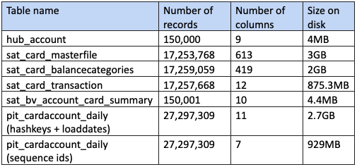
With the above table statistics, the below are the statistics produced when joining the four satellite tables to deploy a virtual information mart.

1) Without a PIT, 2) With a PIT using HashKeys & LoadDates, 3) With a PIT using Seq-ids

Without a PIT table the query run time was nearly 8 and half minutes! Note the volume of data scanned over the network.
A PIT table with hash keys and load dates reduced the query time down to 20 seconds with far less network traffic, a saving of over 8 minutes.
A PIT table with sequence ids halved the above byte numbers and shaved off a further 5 seconds in query time.

NOTE: All the above tests were conducted with RESULTCACHE turned off, an XSMALL virtual warehouse which was flushed between run tests. The results are consistent.

Part 1 of 2 on query optimization

Recognizing that Snowflake has an OLAP query engine is the first step to understanding how to design efficient data models and identifying when query assistance tables can be used to improve the performance you get out of your Data Vault on Snowflake.

In the next blog post we will discuss another technique that will greatly improve query times for very large satellite tables (those with sharp eyes may have seen this technique already being used in the above star optimized query). Until next time!

References:

Originally posted on August 29, 2022 @ 2:00 pm